Rebecca Feng and Austin Zhu
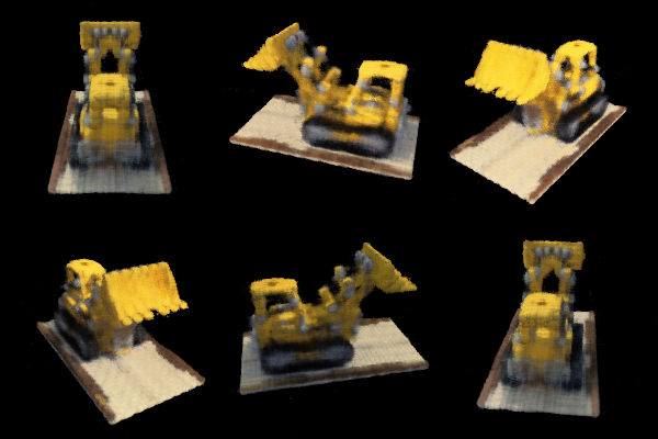

We can reconstruct a scene in 3D given only a series of images that capture the scene, along with each image's associated camera extrinsics and intrinsics. One method of scene reconstruction is through neural radiance fields (paper here), which, given an arbitrary camera position and rotation, can reconstruct an image view by calculating each pixel's color and density. For scene reconstruction, we first break down each training image into varying frequency levels via positional encoding, then train a model to generalize this to predict the corresponding colors and densities at any arbitrary camera position and rotation.
To motivate the idea of using positional encoding to reconstruct images in 3D, we first look at a simpler 2D case and create a "neural field". We attempt to reconstruct images with positional encoding, which predicts RGB values based on 2D image coordinates $x = (u,v)$. We use $L$ to denote the maximum frequency we compute the positional encoding of $x$ for. The equation to break a coordinate $x$ down to its higher-dimensional positional encoding representation is given by:
\[ PE(x) = \{x, sin(2^0\pi x), cos(2^0\pi x), sin(2^1\pi x), cos(2^1\pi x), ..., sin(2^{L-1}\pi x), cos(2^{L-1}\pi x)\} \]Afterwards, we can train an image to predict the rgb color of an image given its image coordinate $x$ using the following multi-layer perception network:

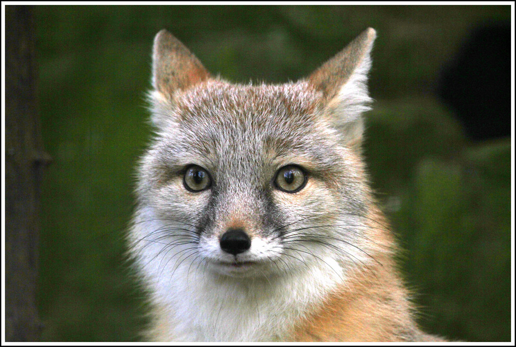
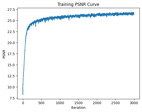
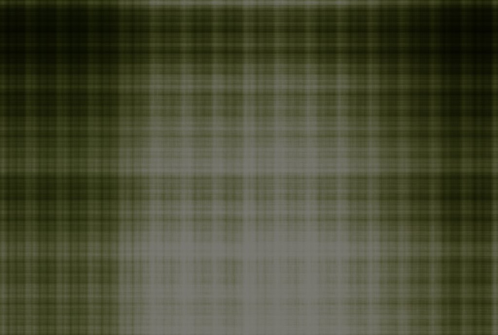
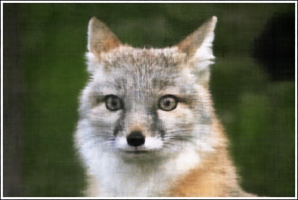
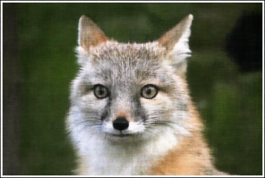
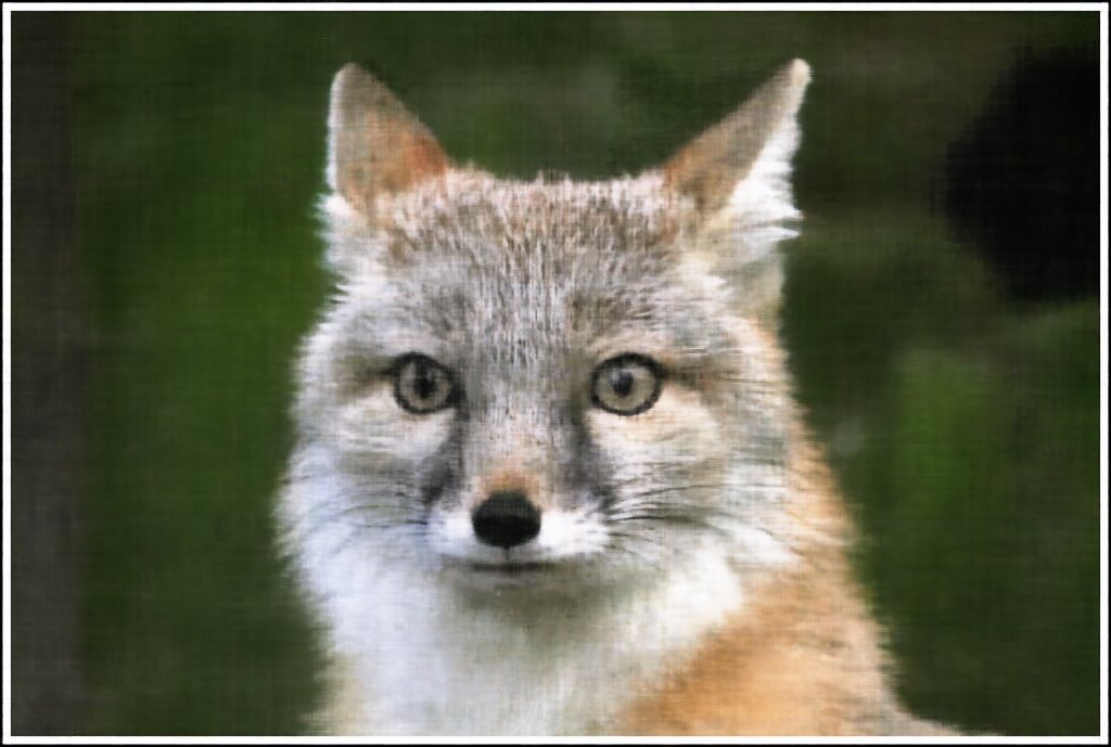
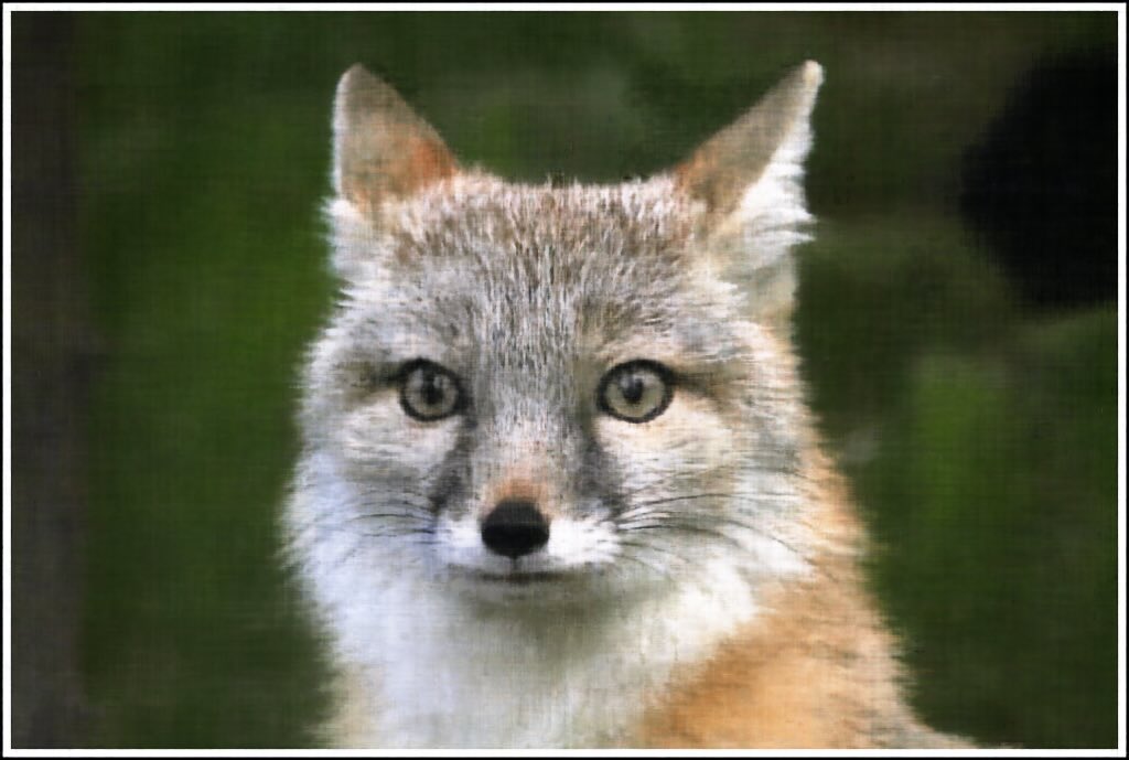
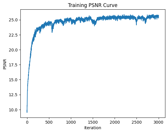
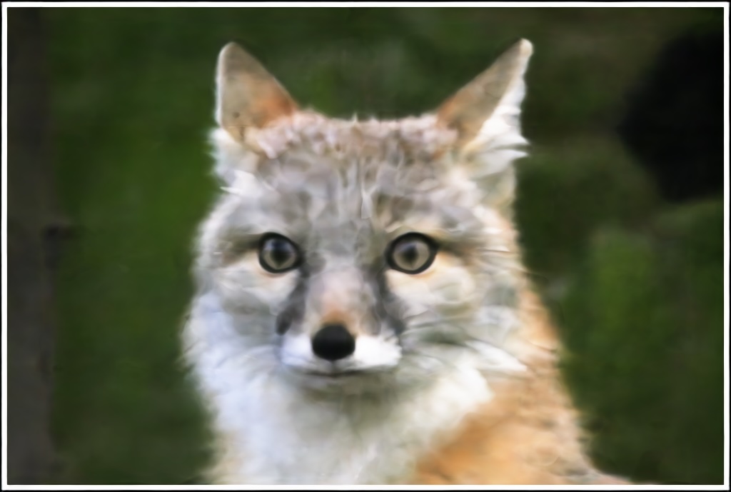
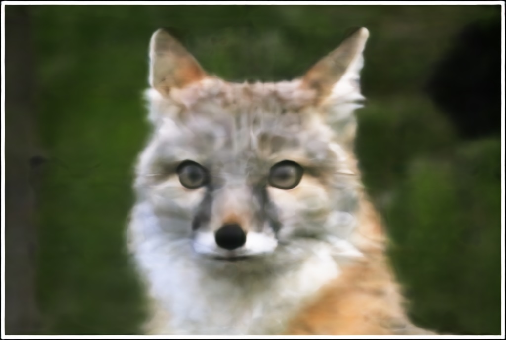
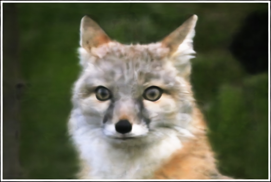
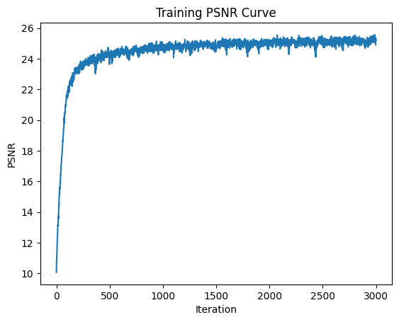
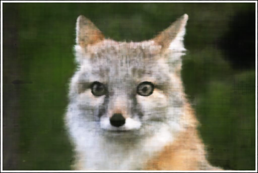
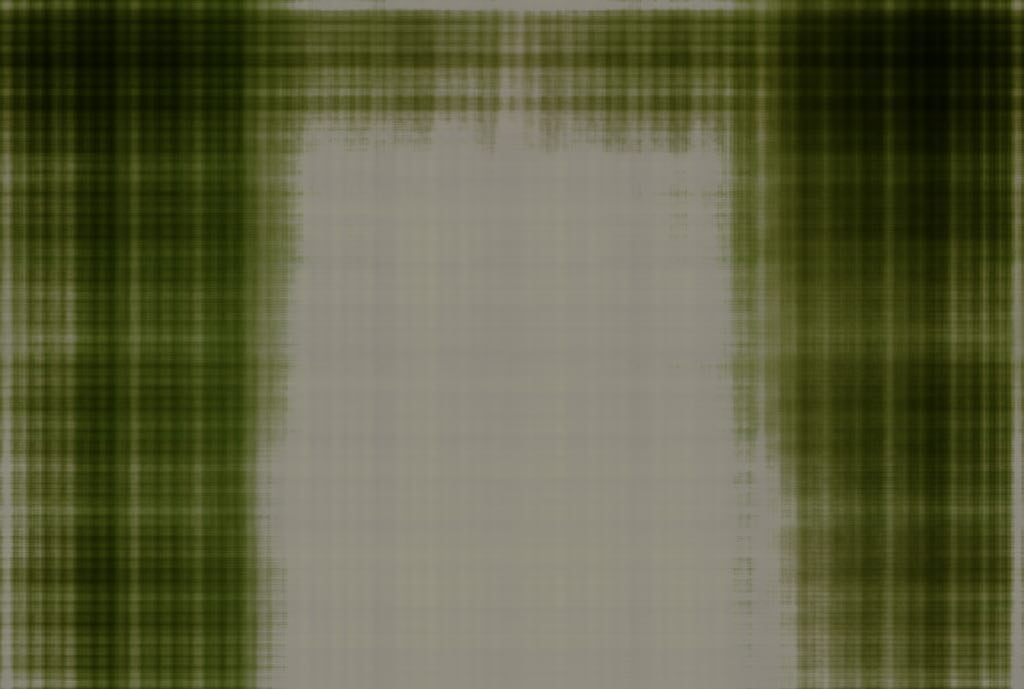
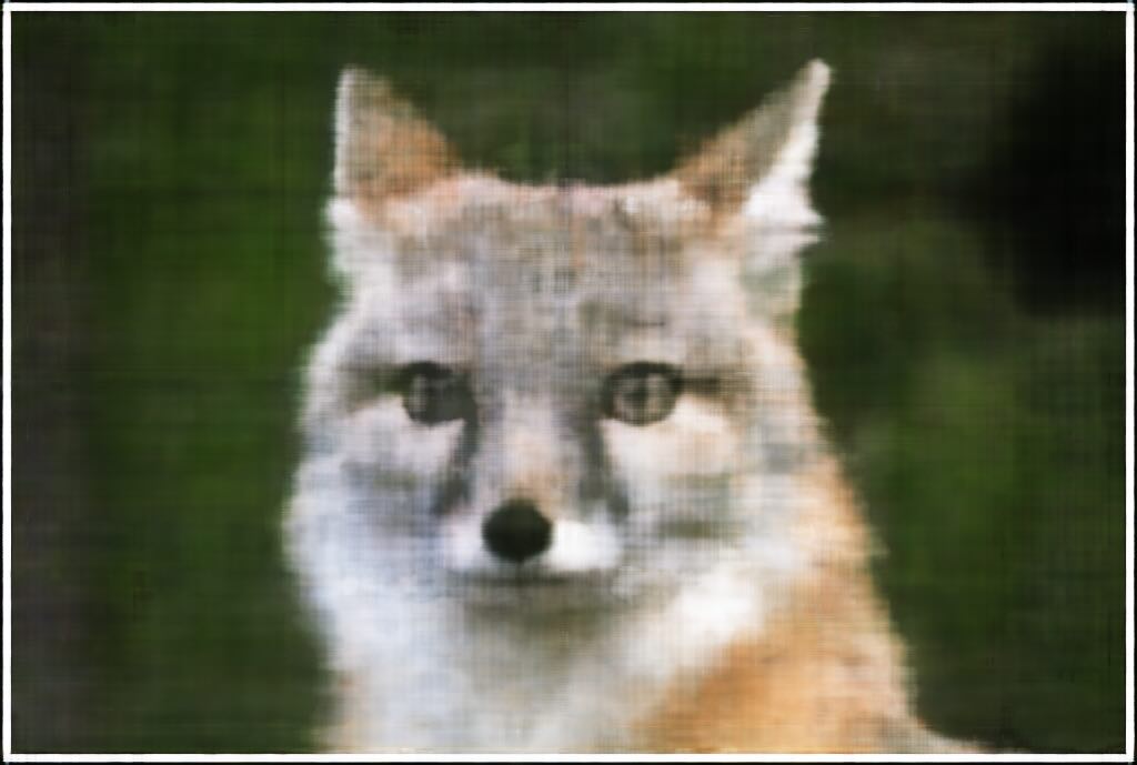
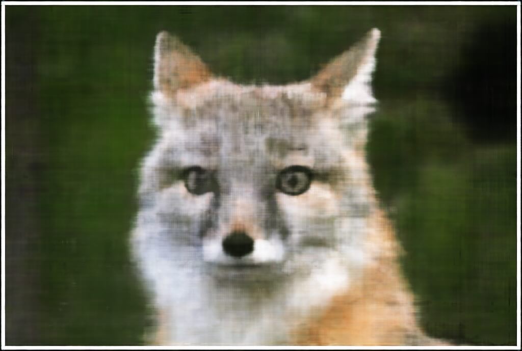
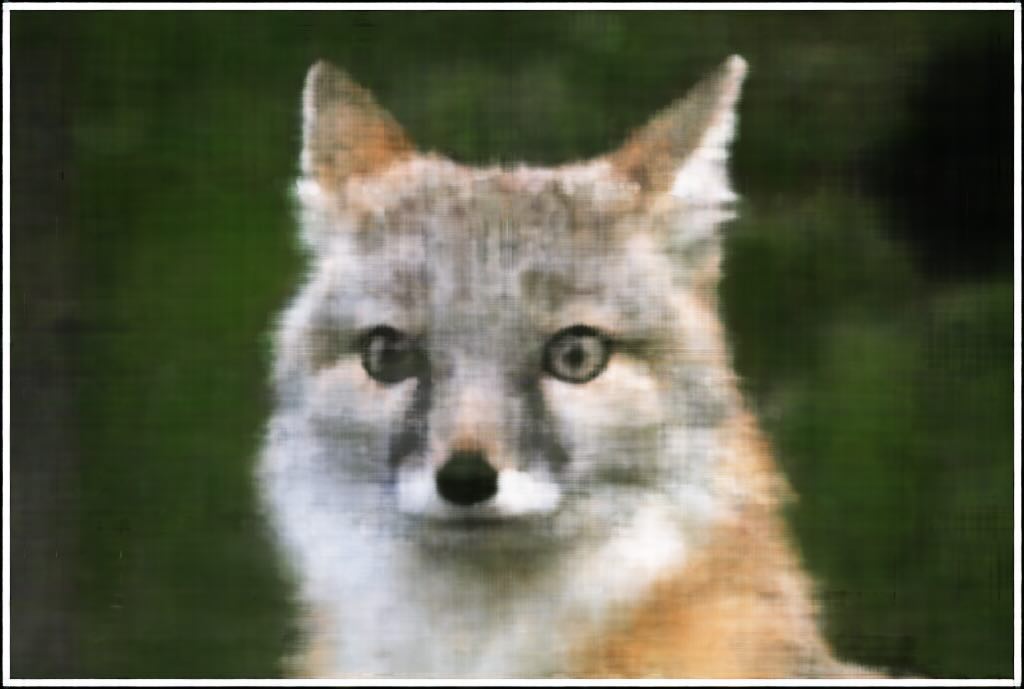
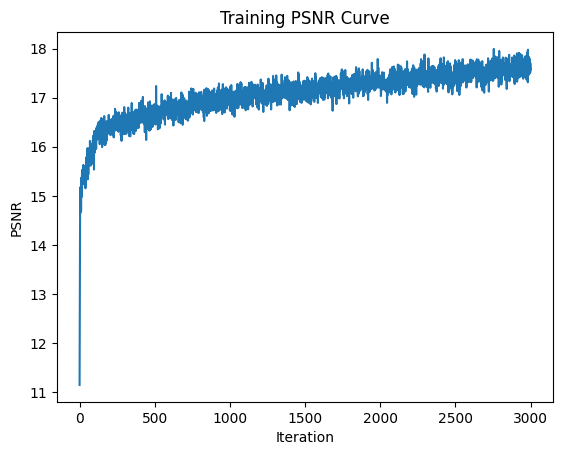
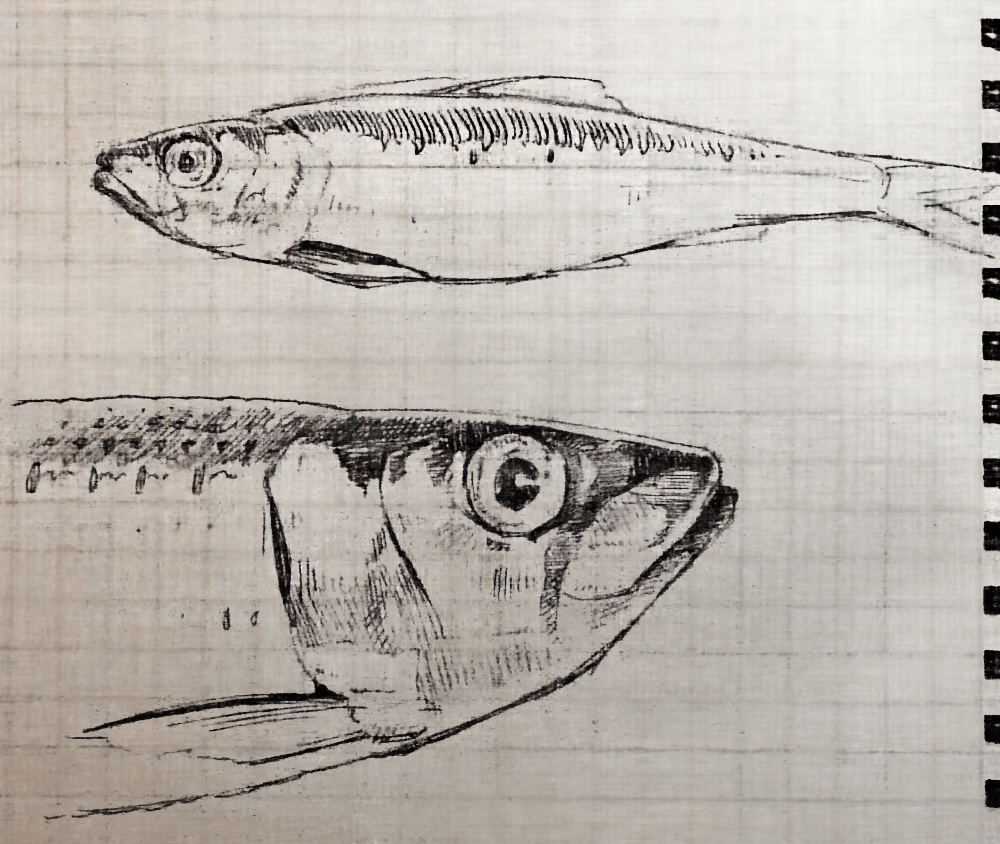
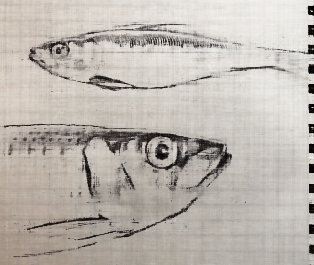
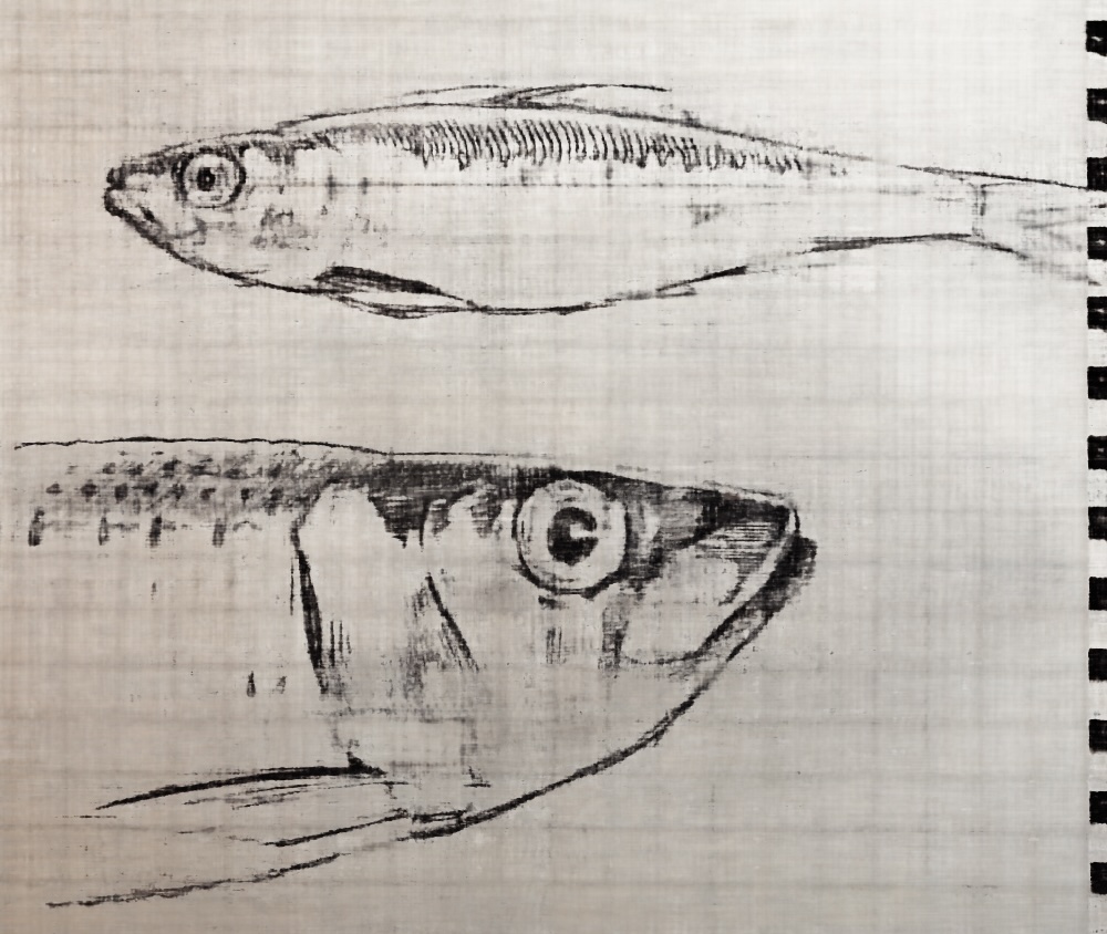
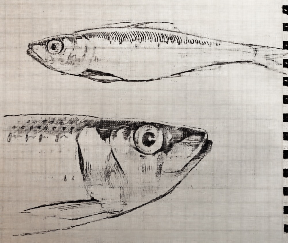
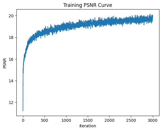
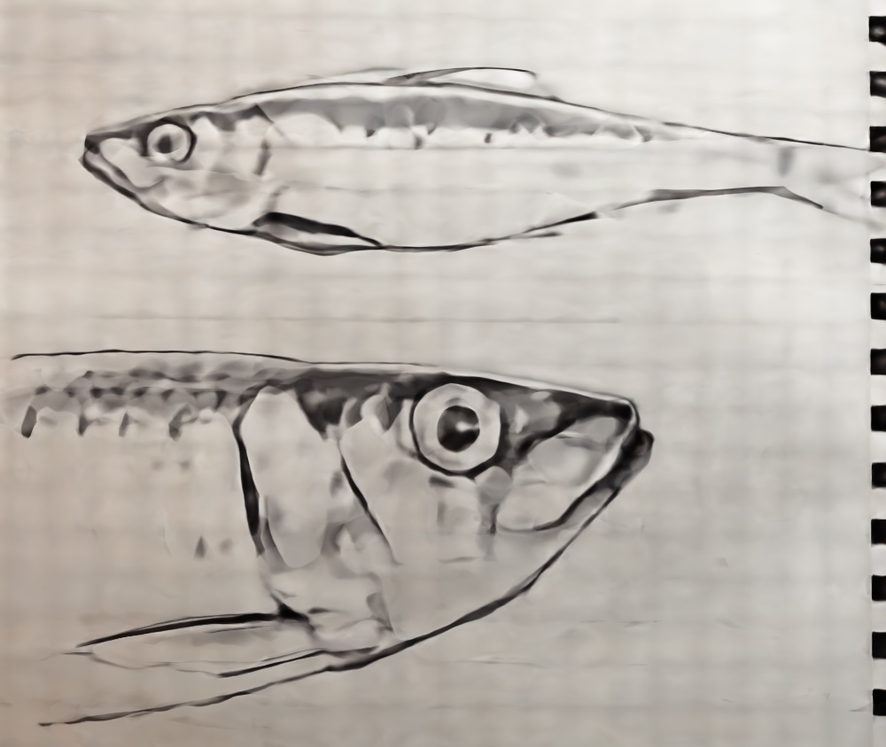
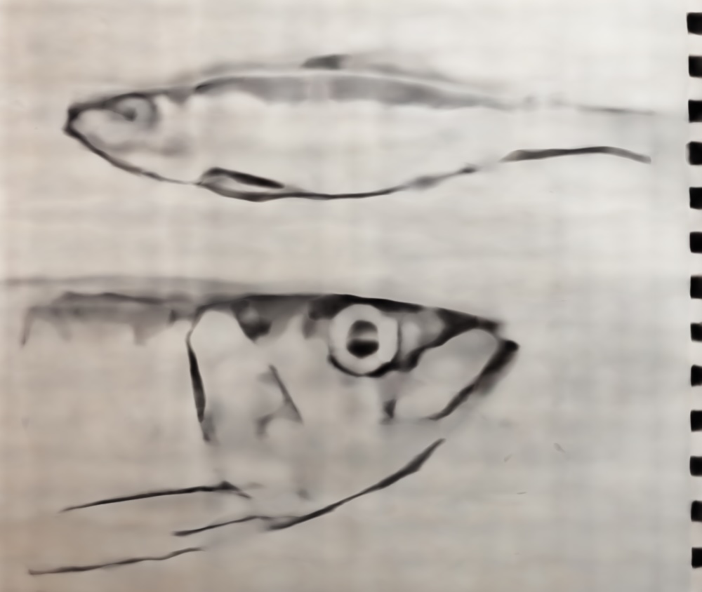
Here are several results of image reconstruction. To start, we train with the following parameters: MSE loss, Adam optimizer 0.01 learning rate, 10000 batch size of pixel coordinates, 3000 iterations, 256 hidden layers, 10 positional encoding levels. Then, we compare the quality of our result by modifying the number of positional encoding levels to 5, and the number of hidden layers to 64, separately. We notice that higher levels of positional encoding levels and hidden layers result in higher quality.
|

|
|
|
|
|
|
|
|
|
|
|
|
|
|
|
|
|
|
|
|
|
|
|
|
|
|

|
|
|
|
|
|
|
|
|
|
|
|
|
|
|
|
|

|
|
|
|
|
|
|
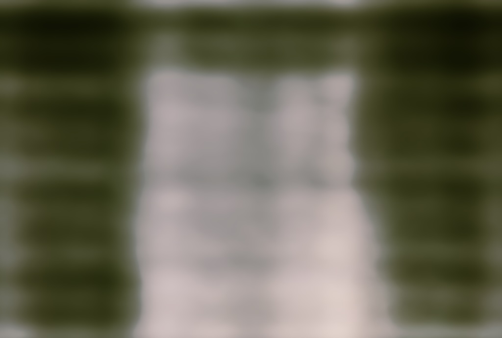
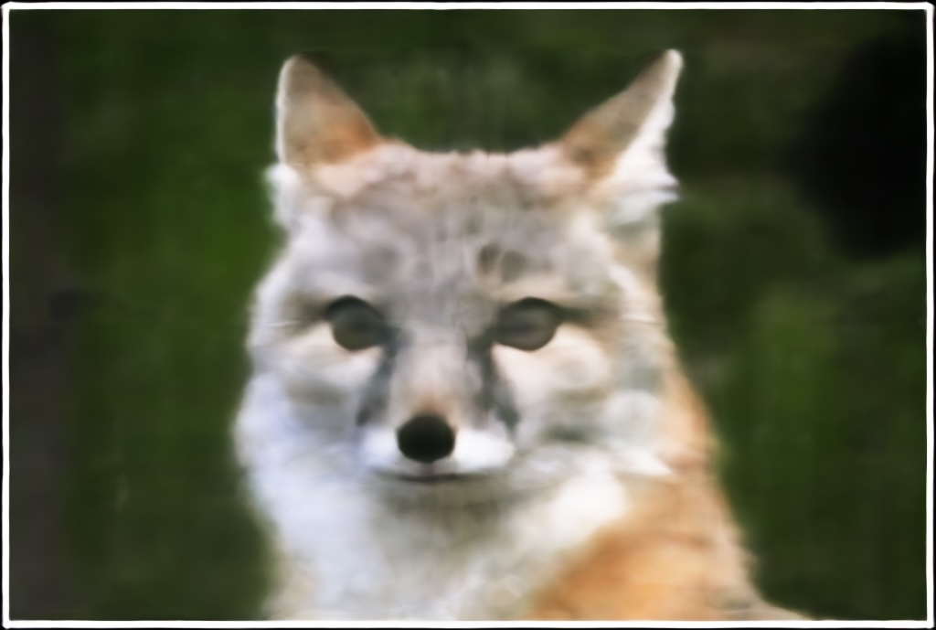
Here, we vary the positional encoding levels from 1 to 5 to 10 and compare the quality of the final reconstructed image. As expected, higher levels of positional encoding (that allow us to retain higher frequency positional accuracy) results in higher quality reconstruction, and more parameters allows us to put in more information in order to generalize our reconstruction.

|
|
|
|
|
|
|

|
|
|
|

|
|
|
|
|
|
|
|
|
|
|
|
|

|
|
|
|

|
|
|
|
|
|
|

|
|
|
|
|
|

|

|
|
|

|
|
|
|
|
|
|
Now, we bring our ideas of image reconstruction to 3D in order to generate neural radiance fields. Firstly, we need to deal with image projections in 3D space, a.k.a., map world coordinates $(x_w, y_w, z_w)$ in 3D space to 2D pixel coordinates $(u,v)$ in image space. We create a matrix that converts an arbitrary world coordinate in 3D to a pixel coordinate on an image, and its inverse to convert image coordinates into world coordinates:
\begin{equation} \begin{bmatrix} u \\ v \\ 1 \end{bmatrix} = w2c * K^{-1} * \begin{bmatrix} x_w \\ y_w \\ z_w \end{bmatrix} \end{equation}where $w2c$ is the world to camera transformation matrix and $K$ is the pixel to camera matrix. \begin{equation} K = \begin{bmatrix} f_x & 0 & o_x \\ 0 & f_y & o_y \\ 0 & 0 & 1 \end{bmatrix} \end{equation} \begin{equation} w2c = \begin{bmatrix} \mathbf{R}_{3\times3} & \mathbf{t} \\ \mathbf{0}_{1\times3} & 1 \end{bmatrix} \end{equation}
Furthermore, $w2c$ is the transformation matrix between homogeneous world and camera coordinates $(x_w, y_w, z_w, 1)$ to $(x_c, y_c, z_c, 1)$ respectively, and in the equation above, we implicitly remove the extra dimension from the homogeneous camera coordinates before applying the camera to pixel transformation $K^{-1}$ deleted.
The other way around, from pixel coordinates to world coordinates, we can simply invert the matrices:
\begin{equation} \begin{bmatrix} x_w \\ y_w \\ z_w \end{bmatrix} = c2w * K * \begin{bmatrix} u \\ v \\ 1 \end{bmatrix} \end{equation}where
\begin{equation} c2w = \begin{bmatrix} \mathbf{R}_{3\times3} & \mathbf{t} \\ \mathbf{0}_{1\times3} & 1 \end{bmatrix} ^{-1} \end{equation}In 3D world coordinates, a ray is specified by an origin, and a direction. Given an origin coordinate $r_o$ and another direction coordinate $r_d$, we can draw rays extending from our camera to our scene view. For a given camera, our $r_o$ and $r_d$ are calculated as:
\begin{align} \mathbf{r}_o = -\mathbf{R}_{3\times3}^{-1}\mathbf{t} \end{align} \begin{align} \mathbf{r}_d = \frac{\mathbf{X_w} - \mathbf{r}_o}{||\mathbf{X_w} - \mathbf{r}_o||_2} \end{align}Together, we can calculate a ray from pure image coordinates by placing the origin ray 1 unit away from the image plane, so that the world coordinate of the image pixel represents the direction of the ray.
Once we have our rays, we would like to sample along the ray so that we can calculate the color and density of a 3D volumetric representation. The volume rendering equation is:
\begin{align} C(\mathbf{r})=\int_{t_n}^{t_f} T(t) \sigma(\mathbf{r}(t)) \mathbf{c}(\mathbf{r}(t), \mathbf{d}) d t, \text { where } T(t)=\exp \left(-\int_{t_n}^t \sigma(\mathbf{r}(s)) d s\right) \end{align}Because it is computationally intractable to to get the color at every infinitesimal $dt$ along the ray $\textbf{r}(t)$ with this integral, we discretely approximate it to:
\begin{align} \hat{C}(\mathbf{r})=\sum_{i=1}^N T_i\left(1-\exp \left(-\sigma_i \delta_i\right)\right) \mathbf{c}_i, \text { where } T_i=\exp \left(-\sum_{j=1}^{i-1} \sigma_j \delta_j\right) \end{align}Thus, we sample along the ray with a near clipping plane of 2 and a far clipping plane of 4. We attempt to get a uniformly random distributed set of sample points along the ray, by first getting 64 samples with a step size of (6 - 4) / 64 then perturbing each sample along the ray uniformly within 0.02 units in order to avoid overfitting when training.
We created a dataloader that generates 10000 random rays when you initialize it with a set of images. Here, we randomly sample N rays extending from a randomly sampled M images, with 64 samples along each ray, rendered in Viser:
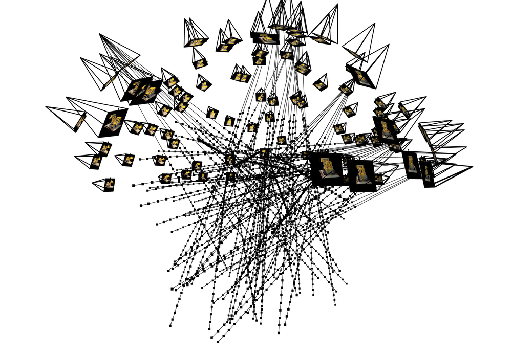
Similar to part 1, we would like to take as input a 3D coordinate and output a predicted color in rgb and its density at that point. We create a neural network, inputting in a 3D coordinate and positionally encoding it. At some intermediary step, we also posiitonally encode the ray direction and insert it into our model. Here is the architecture:

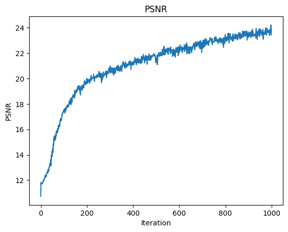
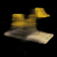
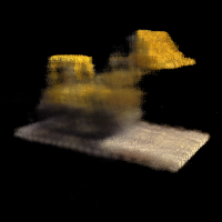
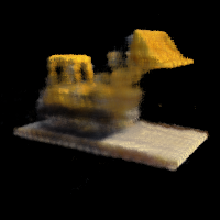
Initially, we trained on 1000 iterations with a learning rate of 0.0005 on an Adam optimizer, with a MSE loss comparing the pixel values of our predicted image view with the original image input, and 10 positional encoding levels. There are 64 samples along each ray for volumetric rendering.
For ray sampling, we randomly sampled, with replacement, 10 images at a time, with 10000 rays in a batch. We uniformly sampled pixels over all 10 images at a time (i.e. 1000 rays per image). However, the resulting PSNR levels were relatively low, so we decided to sample over all 100 images at once (i.e. 100 rays per image). Our PSNR levels went up, but still lower than staff's.
Eventually, we decided to use a learning rate of 0.001, which, for 1000 iterations, improved the PSNR ~3 levels more. We reached a final PSNR level of 23.856! Better than staff solution.
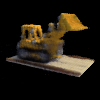
Furthermore, we managed to cut down our training time from 1 hour to 10 minutes. Here are some things we optimized on:
|
|

|
|
|
|
|

|
|
|
|

|
|
|
|
|
|
|
Here's an Autodesk Maya plugin that Rebecca made for Nerfstudio. Essentially, it computes the corresponding camera extrinsics and intrinsics with respect to the mesh representation of the NeRF in Maya for every animation frame, and writes a camera path json file that can be opened and processed in Nerfstudio to render scenes, allowing the user to combine animations in Nerfstudio and in Maya! Here is a small animation combined with Cyrus Vachha's Doe Platform Sundown dataset. Taking a character asset from the 3D Modeling and Animation at Berkeley club ( which Rebecca sculpted), she composited the rendered animation with the nerf scene using the plugin. Still have to reformat some code but here's the pull request and link to download