
|


|


|
Modifying an image by creating filters and separating out its frequencies can give some stunning results, such as getting its edges or seamlessly blending two images together to make it appear as one. This project explores the technical details behind processing images via frequency analysis and filtering used in modern photo-editing today.
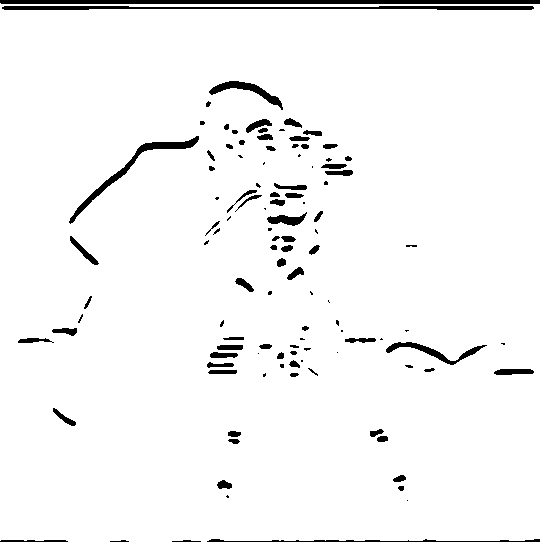
We would like to display the edges of the image below:
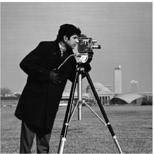
We can do so by using a "finite difference operator." Essentially, we construct horizontal (x) and vertical (y) arrays
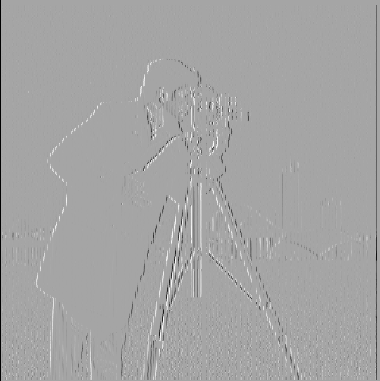
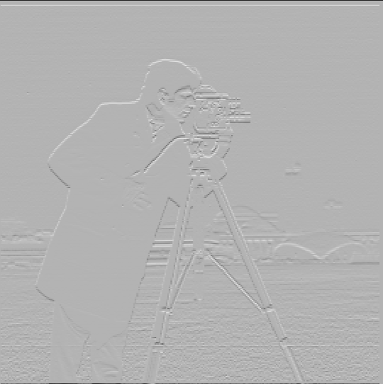
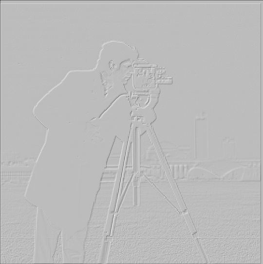
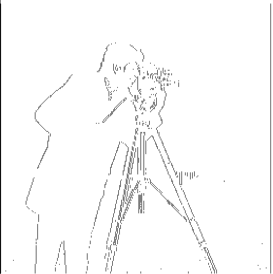
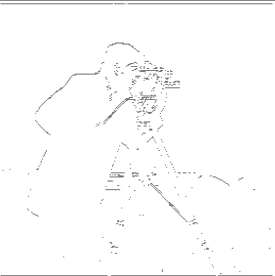
\[ \mathbf{D}_x = \begin{bmatrix} 1 & -1 \end{bmatrix} \quad \mathbf{D}_y = \begin{bmatrix} 1 \\ -1 \end{bmatrix} \]and convolve them around the given image (in this case, the cameraman). Through this convolution, we can compare one pixel in the image to its neighbors. If the two pixels we are comparing have a large difference in value, then the convoluted pixel would be darker. Or if the two pixels are similar in value, then the convoluted pixel would be lighter. Then, the output image after convolution would show up as a series of lighter and darker pixels, where the darker pixels refer to parts of the image with higher contrast with neighboring pixels, creating edges.
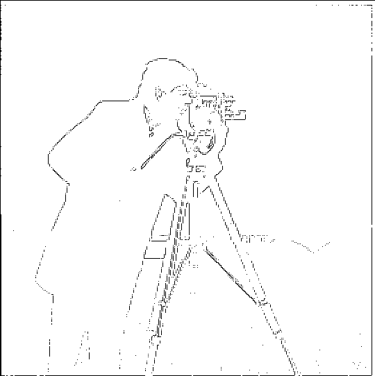
With D_x, we can better see the edges vertically, because the convolution compares one pixel with another to its right/left. With D_y, we can better see the edges horizontally, because the convolution compares one pixel with another above/below. We convolute the image with D_x and D_y then add them together to get the entire edge-detected image.
To display the edges more clearly, we can apply a boolean filter that makes all the edges black, and everything else as white.
|
|
|
|
|
|
|
|
|
|
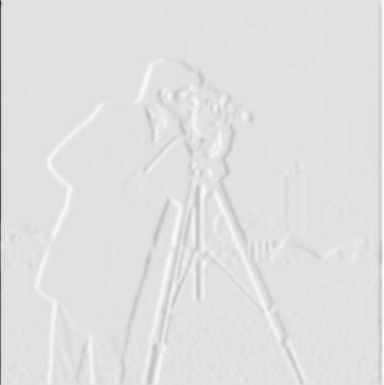
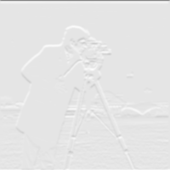
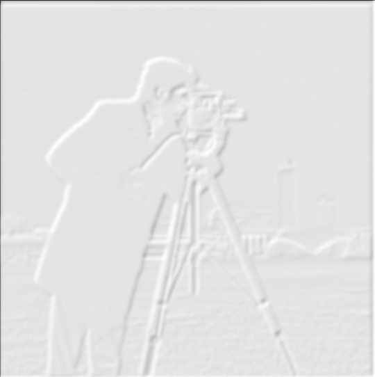
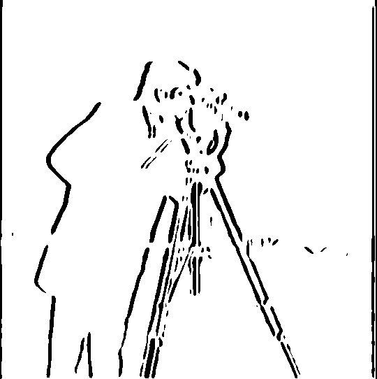
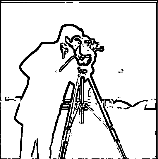
Our results above seem quite pixelated or aliased. Let's see if we can do better by convoluting a Gaussian filter on the image before convoluting it with the final difference operators. We create a 15 by 15 Gaussian kernel with a standard deviation of 15/6, then apply finite difference operators D_x and D_y. Here are the edge results:
|
|
|
|
|

|
|
|
|
|
These results appear much bolder and less aliased than the previous. Additionally, the edges really emphasizes the contours of the man and camera.
Let's compare our results with a single convolution instead of doing the Gaussian kernel and the finite difference operator separately. Here is the new result compared to the one from two separate convolutions:
|

|
They appear the same! This means that performing a single convolution on an image with a Gaussian * finite difference operator kernel is the same as convoluting the image with the kernels separately (Any small inconsistencies between the two images could be due to floating point errors).
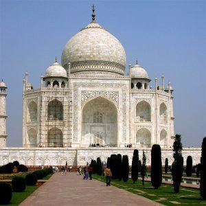
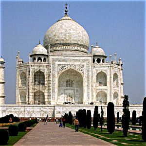
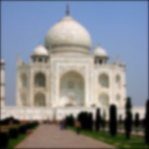
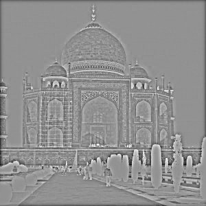
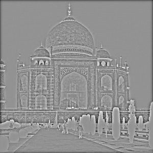
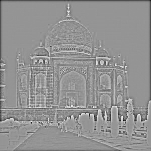
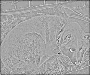
We can sharpen an image by emphasizing its higher frequencies. In order to obtain the high frequencies, we can subtract the original image by all of its lower frequencies. We can get the lower frequencies of an image by convoluting it with a Gaussian kernel. Then, we add our isolated higher frequencies back onto the original image to yield the following results:
|
|

|
|
|
|
|
|
|

|
|

|
|
|
|

|
|

|
|
|
|
|
|
|
|
|
|
|
More formally, the equations to obtain a sharpened image are listed below. For the Taj Mahal, we used alpha = 0.75 and a Gaussian kernel of size 15 by 15 with standard deviation 15 / 6.
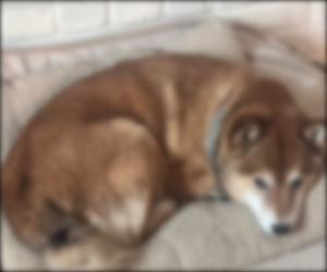
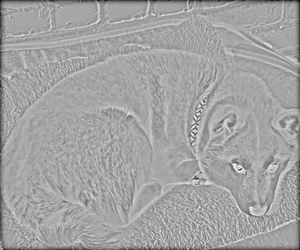
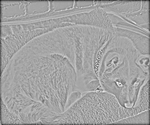
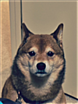
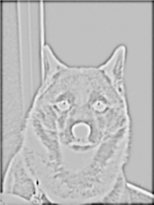
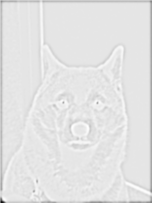
\[ f_{high} = f_{original} - f_{blurredimage} \quad \] \[ f_{sharpenedimage} = f_{original} + \alpha f_{high} \]For experimentation, let's try to restore a blurred image to its original using this technique. We take an image, blur it, sharpen the blurred image and compare it with the original. Here are the results:

|

|
|
|
|
|
|
|

|
|
|
|
|
|
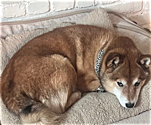
Although the sharpened blurred image does not look as great as the original, we were able to restore a few details in the blurred image, such as the specularity in the dog's eyes or the grainy texture of the carpet.
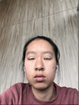
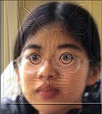
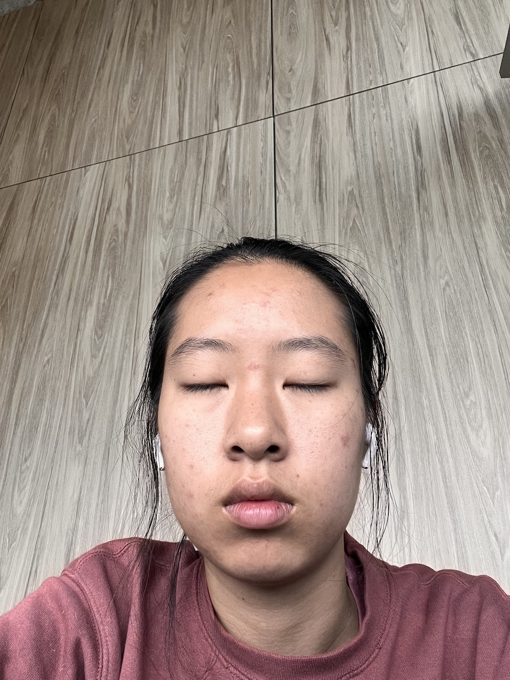
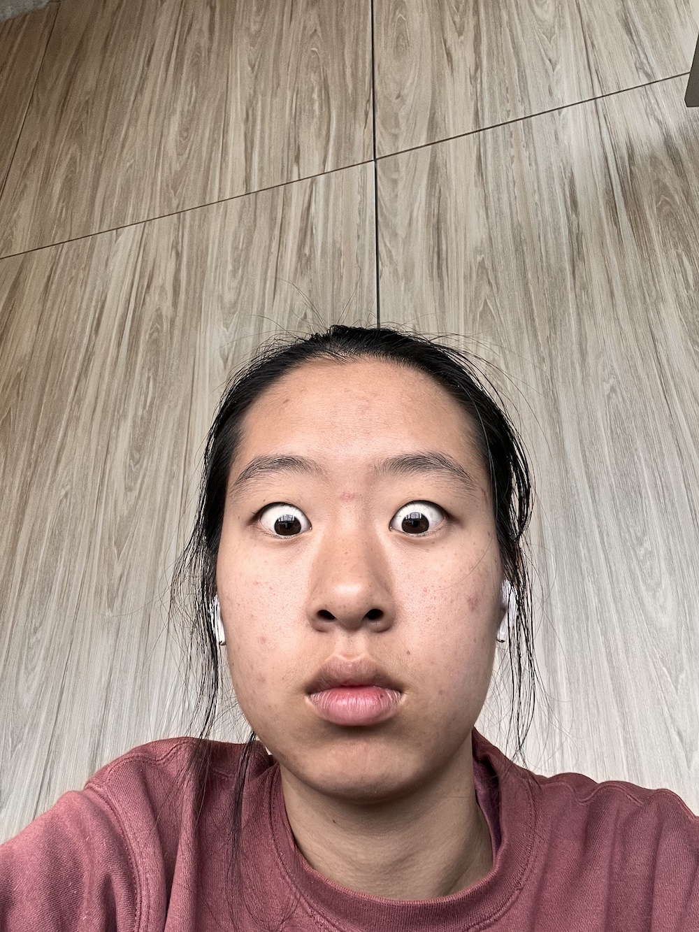
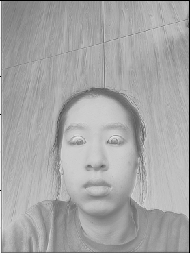
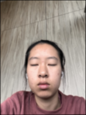
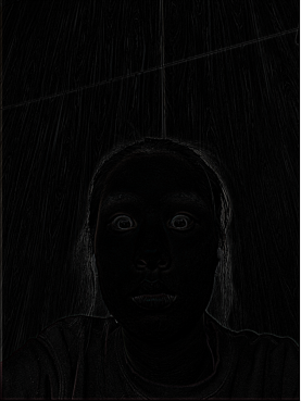
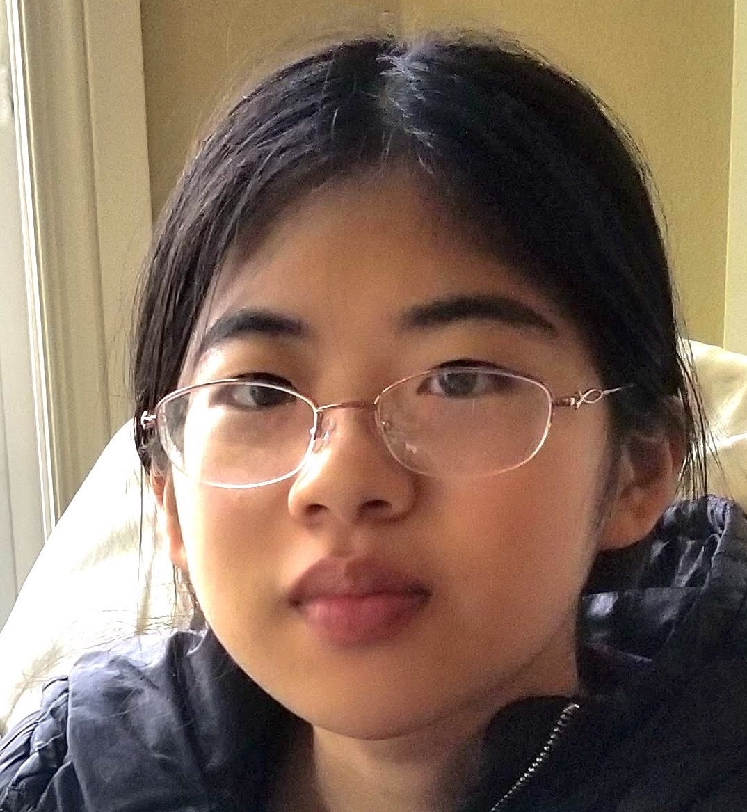
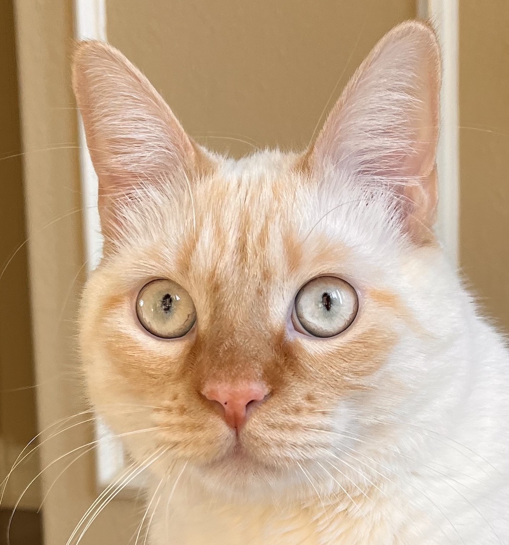
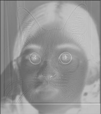
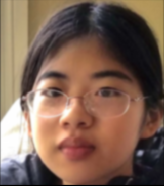
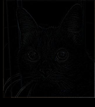
We can leverage this sharpening technique described above to make some fun optical illusions. From close up, you will see the higher frequencies of an image better than the lower ones. From far away, the lower frequencies will dominate the perception of the image. We can combine the high frequencies of one image, and the low frequencies of another so that up close, the combined image will appear as one thing, and far away, it will appear as something completely different. Here are some results:
|
|
|
|
|
|
|
|
|
|
|
|
|
|
|
|
|
|
|
|
|
Comparing the colorized vs the black and white results, we can see that the black and white results give a better read of the seeing the high frequency image up close, and the low frequency image far away. In the colored version, the colors from the low-frequency image can be very distracting when trying to view the high frequencies up close.
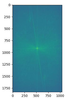
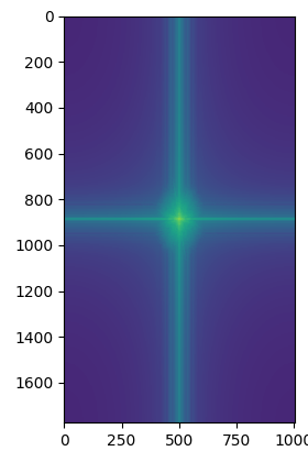
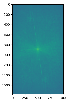
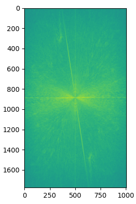
When we create a low pass image via a Gaussian kernel, we get rid of all the high frequencies of the image. Likewise with the high pass, we get rid of the low frequencies of the image. We can illustrate this by displaying the Fourier transform of the "Rebecca is awake AND asleep" result.
|

|
|
|
|
|
|
|
|
|
|
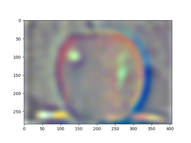
This hybrid image did not go too well. Even at high frequencies, the text appeared as normal. From far away, the high pass text still appeared quite distinctly from the resulting image, and it is hard to read what the text says in the low-pass. However, the penguin blended in pretty well.
|
|

|
|
|
|
|
|
|
|
|
|
|
|
|
|
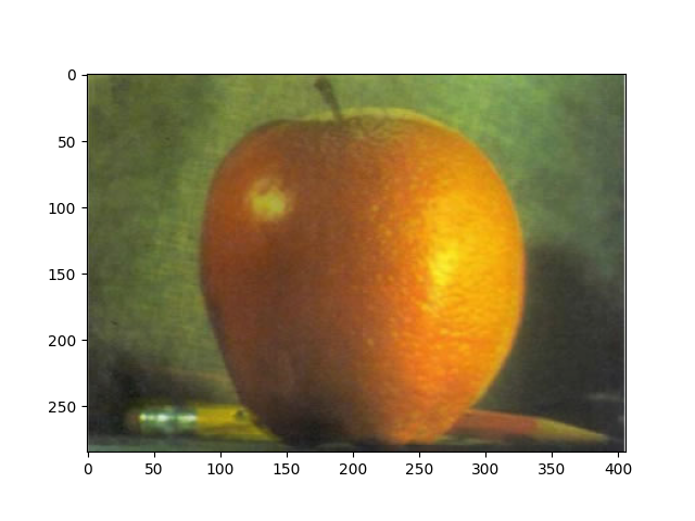
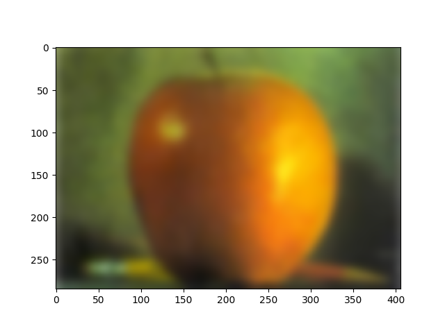
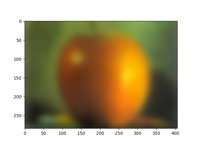
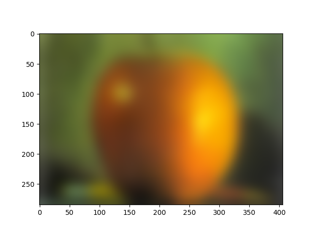
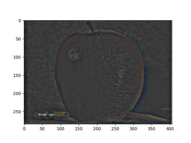
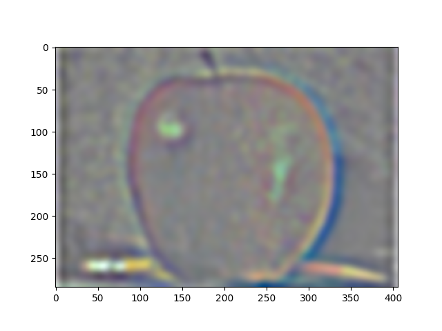
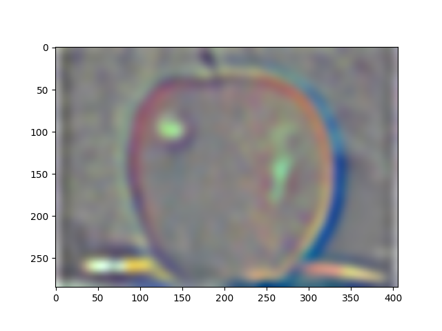
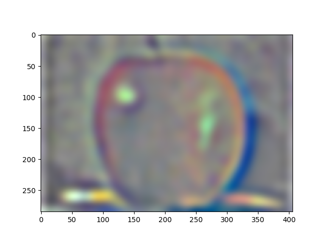
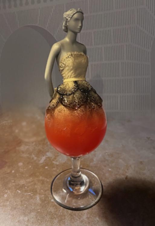
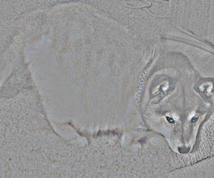
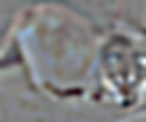
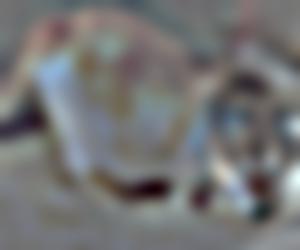
We used the techniques described by the 1983 paper by Burt and Adelson to seamlessly blend one image with another. We compute the Laplacians, or get the band pass, of the image to separate the frequencies of the image. The last level is simply a Gaussian of the image, blurred the last level number amount of times. From there, we can individually blend together each band pass together with the corresponding level's mask, and add together all of the blended images into one. Here are some results using a vertical mask and a horizontal mask respectively:
|

|
|
|
|
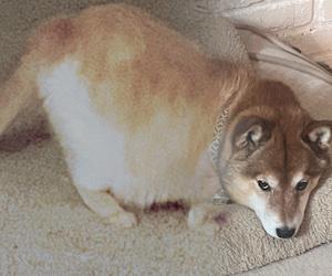
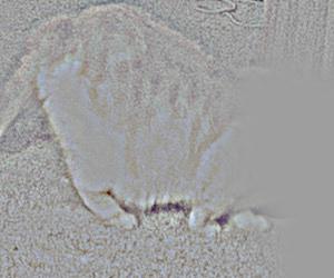
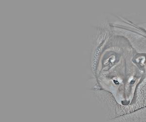
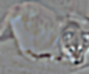
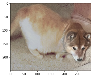
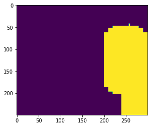
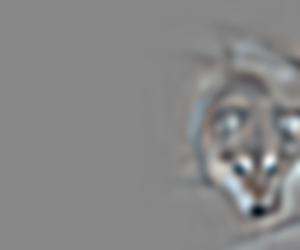
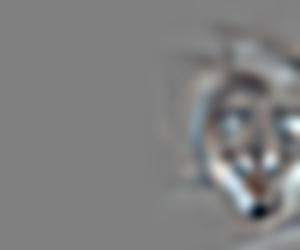
For the dogcat, I also implemented a custom mask, where we only take the dog's head and blend it with the cat photo, as opposed to the previous implementation which used a horizontal mask instead. Here are the results and the corresponding Laplacian masks. Additionally, we align each mask level used for the dog and cat Laplacians.
|
|
| Blended |
|

|
|

|
|
|
| Masked cat |

|
|

|
|
|
|
| Masked dog |

|
|
|
|
|
|
| Masks |

|
|

|

|
|
|
| Stack levels |
|
|
|
|
|
|
That's it folks