Rebecca Feng
Part A: The Power of Diffusion Models!
0. The DeepFloyd Diffusion Model
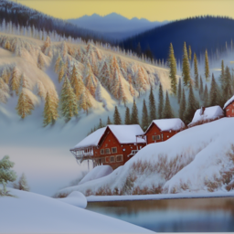
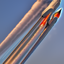
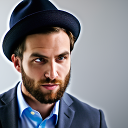
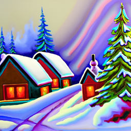
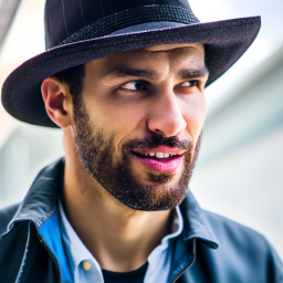
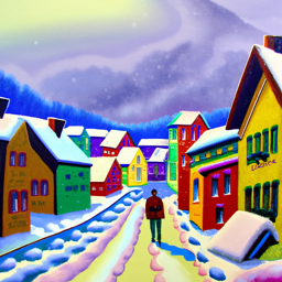
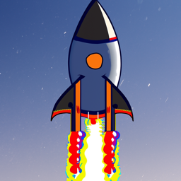
Let's test out the diffusion model by inserting some prompts! We notice that the higher step count we have, the higher the quality of our images, and the more accurate the image is to the prompt. We are using a random seed of 180.
| Step size | A man wearing a hat |
An oil painting of a snowy mountain village |
A rocket ship |
| 2 |
|
|
|
| 5 |
|
|
|
| 10 |
|
|

|
| 20 |
|
|
|
1. The Forward Process
The forward process in diffusion models consists of taking an image, and adding noise to it. The resulting noised image at timestep t, denoted as x_t, is given by the equation
t has values ranging from 0 and T. When t=0, we should yield a clean image. When t=T, the image should be maximally noised. The noise in the image is sampled in a normal distribution. Here are the results of the noised test images at timesteps t = 250, 500, and 750:

|

|

|

|
|
|
|
|
|
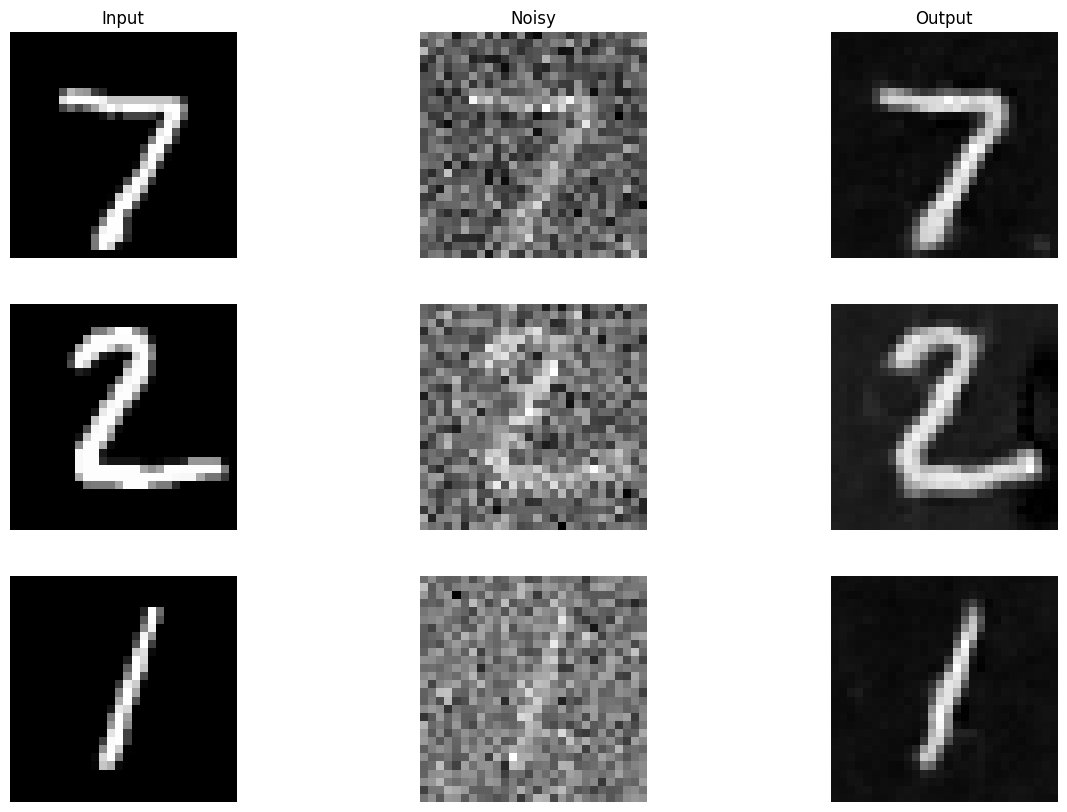
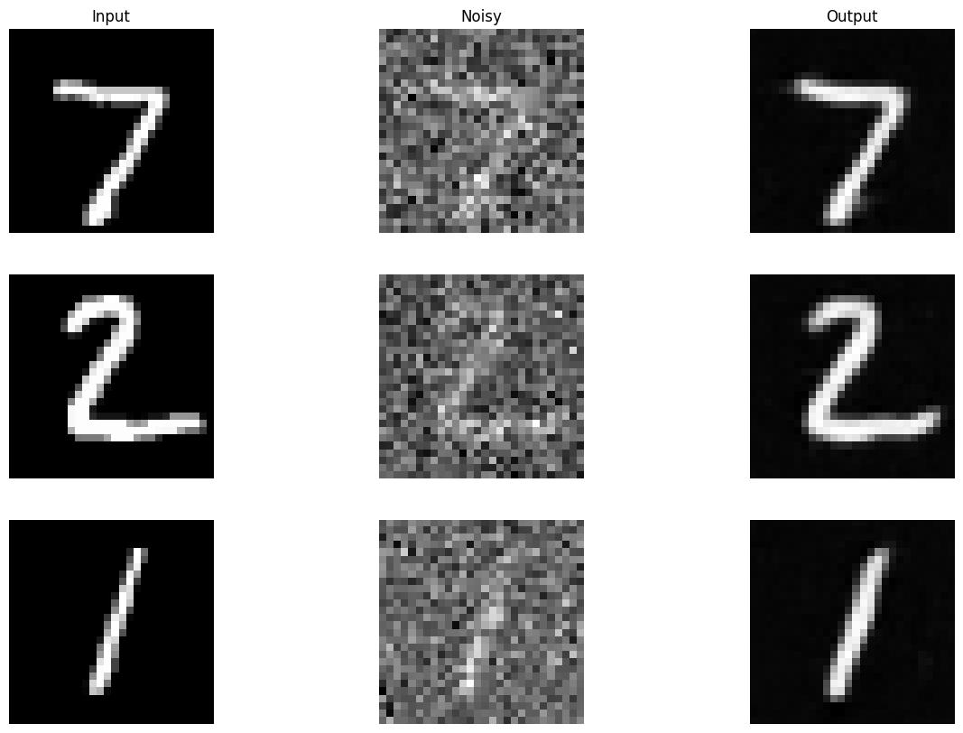
2. Classical Denoising
Now let's try denoising these images. We can attempt to do so by simply doing a Gaussian blur, with a kernel size of (7,7). However, we find that the noisier an image is, the less quality the result:
|
|
|
|
|
|
|
|

|

|

|
|
|
|
|
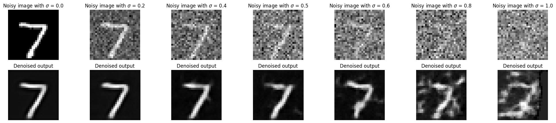
3. One-Step Denoising
We use a pretrained diffusion model to attempt to denoise our
input noised image in one step, with the prompt "a high quality photo". That is, we try to remove the
noise all at once. We use the given unet to predict the noise
in the image, and subtract the noise from our current noised image,
in order to get a denoised one. Here are the results for denoising
an image at varying noise levels.

|

|

|
|
|
|
|
Notice how increased levels in noise make it harder to predict the original image passed in. This makes sense because as an image gets noisier, it is less clear what details are in the original image, so we pull some assumptions about what details might be included in the original image.
4. Iterative Denoising
We can improve our results above by denoising our noised image
step by step, removing a little bit of noise each time in the
direction of our prompt. We create a list of timesteps from
t = 0 to t = 1000. However, having to denoise an image one step
at a time, totaling up to 1000 steps, can be computationally expensive.
Instead, we can skip a few timesteps in each iteration. We keep
track of these skipped timesteps through an array we define as
strided_timesteps, consisting of only every 30th
timestep.
The equation to estimate our less noisy image is
where t' is the next strided timestep leading to a less noisy image, t is our current timestep, x_0 is the current estimate of the original image (predicted in 3), and the alphas are noise coefficients at their respective timesteps. The v_sigma is also some predicted noise.
We show the process of a noised image being iteratively denoised, resulting in a final, less noised, predicted result:

|

|

|

|

|
|
|
|
|
|
|
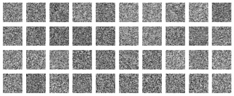
5. Diffusion Model Sampling
With our trained model, we attempt to generate random images of our own now
by passing in random noise, and seeing what the model outputs based upon our
prompt, a high quality photo. Here are some results:

|

|

|

|

|
|
|
|
|
|
|
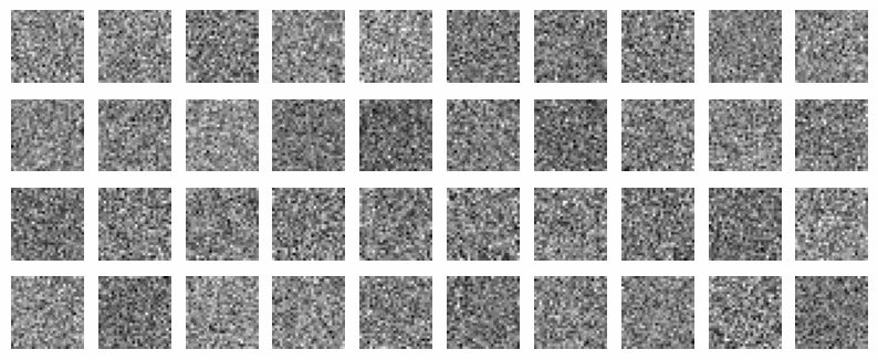
6. Classifier-Free Guidance (CFG)
You may notice that a couple of the images, or parts of the images above seem unclear in what they are depicting. We aim to make the quality of these images better, and have more comprehensible results, by employing a technique called "classifier-free guidance."
We estimate both a conditional noise estimate $\epsilon_c $ and unconditional noise estimate $\epsilon_u $, such that our final output noise is
where $\gamma$ is the strength of the classifier free guidance. We end up having higher quality images when $\gamma > 1$. We implement CFG into our iterative denoiser, with $\gamma = 7$
Here are some results:

|

|

|

|

|
|
|
|
|
|
|
These images look way more clear and comprehensible than the ones generated without CFG!
7. Image-to-image Translation
With CFG, we noise a test image a little, then force it back on the natural image manifold in a certain amount of timesteps. We call this algorithm SDEdit. Here are some results noising our image at various noise levels defined at different starting indices for strided_timesteps:
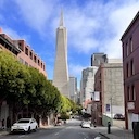
| Campanile |
|

|

|

|

|

|

|
| Ghiradelli Square |
|

|

|

|

|

|

|
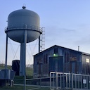
| Water tower |
|

|

|

|

|

|

|
|
|
i_start=1
|
i_start=3
|
i_start=5
|
i_start=7
|
i_start=10
|
i_start=20
|
We can also play around and draw images on our own, or find images on the internet, and pass it through the model to see what the computer predicts the image will end up being:
| Tomato carrot |

|

|

|

|

|

|

|
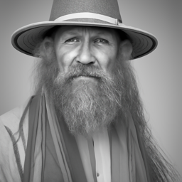
| Mysterious guy |

|

|

|

|

|

|

|
| Galaxy |

|

|

|

|

|

|

|
|
|
i_start=1
|
i_start=3
|
i_start=5
|
i_start=7
|
i_start=10
|
i_start=20
|
We can also perform this algorithm on a portion of our image instead of the entire image. This is called inpainting. We mask out the part of the image that we want to noise and denoise by setting the mask's value to 0 if we want the same content, and 1 if we want to generate something new in the denoising loop.
Here are some inpainting results:
|
|

|

|

|

|

|

|

|
|
|

|

|

|
|
|
|
|
|
Instead of using our default prompt, a high quality photo,
we can change the prompt and generate different looking results combined with
inpainting. We show the result of CFG at different noise levels determined by
i_start and a few chosen prompts:
| A rocket ship |
|

|

|

|

|

|

|
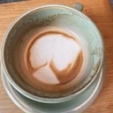
| A photo of a hipster barista |
|

|

|

|

|

|

|
| A pencil |
|

|

|

|

|

|

|
|
|
i_start=20
|
i_start=10
|
i_start=7
|
i_start=5
|
i_start=3
|
i_start=1
|
8. Visual Anagrams
We can also generate optical illusions with our diffusion model. We will generate an image that looks like one prompt when right-side up, but when flipped upside down, it'll look like something else! In order to do so, we generate the predicted noise for the right-side up prompt and the upside-down prompt, average the two, and iteratively denoise our image. Our noise will be calculated as such:
Here are some visual results:
| Right side up |

|

|

|
| Upside down |
|
|
|
| Prompts |
a man wearing a hat |
around a campfire, an oil painting of an old man |
snowy mountain village a lithograph of waterfalls |
9. Hybrid Images
We can also create hybrid images, such that it looks like one prompt looking close up and another prompt looking far away. This is a concept we have explored extensively in earlier projects. High frequencies tend to dominate our interpretation of an image when we look at it up closer, and low frequencies dominate when we look at it far away.
This is how we will calculate the predicted noise at each timestep:
The above calculations for noise are described as follows: utilizing this idea, we predict the noise of the image for prompt 1 at low frequencies-in other words, we take a Gaussian blur of the directly predicted noise from prompt 1 to filter out high frequencies within that noise. For prompt 2, we predict the noise of that image at high frequencies. In other words, we subtract the predicted noise for prompt 1 from the blurred predicted noise for prompt 1 to get only the high frequencies.
We add the resulting noises together to get the predicted noise that we will use for iterative denoising.

|

|

|
|
|
Low freq
High freq |
a photo of a hipster barista |
a lithograph of waterfalls |
a photo of a dog |