This project explores core ray-tracing techniques, particularly in the context of Lambert BRDFs, bounding volume hierarchies, direct and global illumination using Monte-Carlo estimators, and adaptive sampling using 95% confidence intervals.
We generated rays from the camera into the scene, treating the camera as a singular point in space with a virtual rectangular image sensor. For any given pixel in the output image, we generated the same number of rays as the given number of samples. Lastly, we tested these rays for intersection with any objects in the scene using the Möller-Trombore algorithm.
We constructed a BVH out of all the primitives in the scene, using the midpoints of all primitives as a heuristic to split the bounding box into children bounding boxes. We also implemented testing for ray-intersection with a given bounding box, and with any primitives within a given BVH.
We introduce a diffuse BSDF (Bidirectional Scattering Distribution Function) as a basis for rendering direct and global illumination in this and the next part, where an even amount of light is scattered in a hemisphere no matter the direction where the ray hits the surface. Then, we implemented zero-bounce illumination, and one-bounce illumination with uniform hemisphere sampling, and importance sampling lights.
We implement global illumination to get a realistic look to our renders by recursively calling upon one-bounce illumination by the number of times we want the light to bounce. In this implementation, we can also toggle whether or not we want to render an accumulation of all m bounces of light (aka global illumination), or just the mth bounce of light. We also introduce a method for randomly terminating when we want the light to stop bouncing via Russian Roulette, which decreases bias in our global illumination estimate.
The adaptive sampling method we use is a 95% confidence interval on the illumination of the pixel. The idea is that we can dynamically compute the number of samples needed to render a pixel in order to decrease noise, rather than computing a high number of samples for all pixels because some pixels will converge faster with a lower sampling rate than others.
All techniques made use of the provided Ray data-structure, which included information about a particular light ray's origin, direction, maximum depth, and time of intersection, as well as passing in pointers into various methods to fill in information about time of intersection with an object's surface. Debugging was primarily done through visualizing bounding boxes in the GUI, or rendering out the image. Most issues encountered for direct and global illumination had to do with converting between object and world space coordinates, setting small floating-point offsets for the minimum and maximum allowed parameters for ray-intersection, and also a small, but crucial error when determining when a ray intersected through a bounding box.
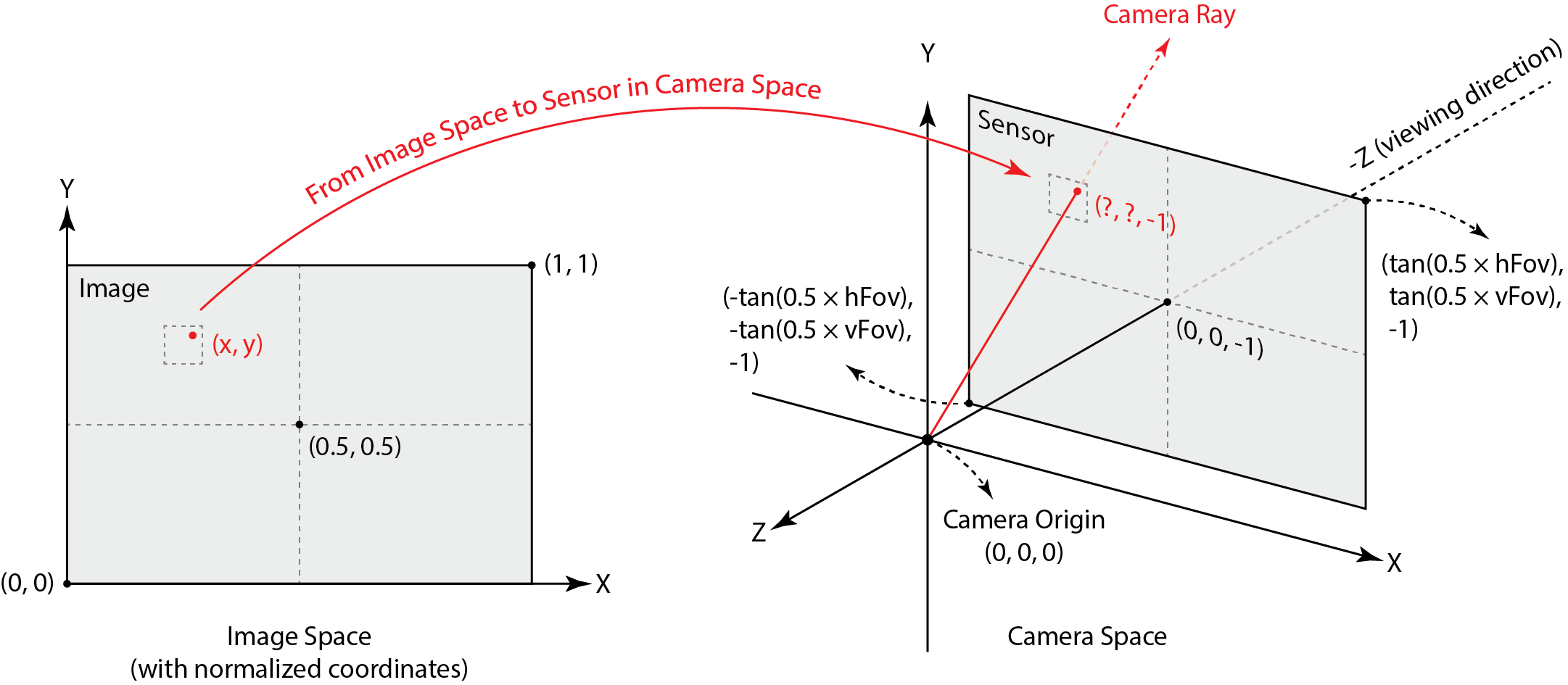
In order to generate rays from a camera pinhole, we had to convert between coordinates from image space to camera space to world space. Given a particular
pixel coordinate in our empty, unrendered image with corners (x,y) = (0,0) and (1,1), we converted to camera space using the given
parameters for horizontal and vertical field of views (variables hFov and vFov for the view angles along the X and Y axis respectively). We also
must take into account the center of the sensor place that lies in camera space (0,0,-1).
The transformation for the image in camera space is represented as:
For any pixel coordinate in image space, we can describe its transformation as:
where the z coordinate is -1 because we offset our camera sensor by -1 with respect to our camera pinhole in the z direction. The transformations can be summarized by the diagram below:
Finally, we normalize the computed direction vector for our ray convert the vector to world space with the provided camera to world matrix, and pass it in with its corresponding origin to the Ray data structure provided. The minimum and maximum values in which the ray can be traced must be defined with the near and far clipping planes of the camera.
For the primitive intersection part of the pipeline, we provided support for intersecting triangles and spheres. Checking for intersection is primarily done via the Möller Trombore algorithm for triangles, and a quadratic form for spheres. For spheres of a given radius R and origin c, and a ray's origin o and direction d, the intersection occurs when
In this quadratic form, we will yield two values for t: t when the ray enters the sphere, and once again when the ray exits the intersection. The smaller value of t will represent when the ray enters the sphere, and the bigger will represent when the ray exits. Because we only care when the ray enters the sphere (we won't see anything behind the sphere). we take the ray's max t value to be the samller value of t. For both the sphere and triangle primitives, once we determine its intersection, we assign its primitives, normal vector from the computed Möller-Trombore parameters, and its BSDF.
For triangle intersection, we take the equation for computing barycentric coordinates in order to see if a ray intersects a triangle given its three vertices, P0, P1, and P2 . We can solve for t, b1, and b2 using Möller Trombore Algorithm where:
From there, normalize the P values and assign other corresponding attributes accordingly.
|
|
|
|
A Bounding Volume Hierarchy (or a BVH) is a data structure that splits primitives into bounding boxes, and
stores these bounding boxes in a tree data structure. The point of a BVH is to ignore all light rays that do
not intersect with the bounding box, because if the ray doesn't intersect with the bounding box, then it won't
intersect with the primitives inside the bounding box. In our BVH tree, we group up to max_leaf_size
number of primitives in a leaf node's bounding box. If a ray DOES intersect with a bounding box, we must
check to see if it intersects with any of the primitives within the box.
In our BVH construction, we start by considering all the primitives in the current bounding box, and also put each
primitive's midpoints in a bounding box. We create a node out of the current list of primitives in our box. The bounding box
would be a leaf node if the number of primitives in it is less than
or equal to the max_leaf_size given. If it is not, we would need a heuristic for
splitting the bounding box in two. Our heuristic was to
split the bounding box in half along its longest axis determined by the midpoints
of the primitives (for example, if the dimensions of our box were 3.0 in the x-direction,
2.0 in the y-direction, and 2.3 in the z-direction, we split the box along the x-direction.
These dimensions are determined by the bounding box of all the midpoints
of each primitive, whether it be a triangle or a circle). After that, we sort the primitives
into two sections, depending on which side of the split they are on. We recursively call BVH
on the two sets of primitives and create future BVH nodes, until all nodes become leaf nodes,
and thus have no children.
|
|
|
|
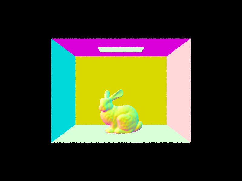
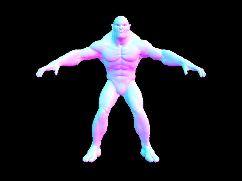
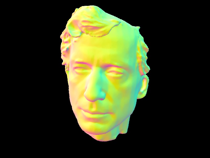
I tested the render times for the cow, Max Planck, and the beast models. Without BVH acceleration, the render times were 34.1616, 349.8426, and 415.8852 seconds respectively. With BVH, the render times were 0.0579, 0.0784, and 0.0488 seconds respectively. From the data given, we can see that using BVH acceleration significantly speeds up our render times, especially for very complex geometry.
There are two direct lighting functions that we implemented: direct lighting hemisphere (generates rays shooting in random directions to sample light in its path) and direct lighting importance (shoots a ray from an intersection point to a light in a list of lights, seeing if there is another primitive in its path).
The objective of the direct lighting function is to define what the outgoing radiance \(L_{out}\) is at a point \(p\) and directional weight \(w_{r}\). Using the Monte Carlo estimator we can estimate the true integral of outgoing light in the following form:
In order to implement this equation, there needs to be a for-loop for each sample. Then, we need to determine the weight of each sample and put it in the world-frame. Based on this information, we can define a ray and an intersection. If there is an intersection, we can apply the above equation.
For the direct lighting with uniform hemisphere sampling, \( L_i(p, \omega_{j}) \) is defined to be amount of light from the new intersection and \( f_r(p, \omega_{j} \rightarrow \omega_{r}) \) is the Bidirectional Reflectance Distribution Function (BRDF). The BRDF describes how light is reflected at \(p\) from \(w_{in}\) to \(w_{out}\).
The other method is importance sampling light which has a slightly different implementation. The main difference in this sampling method is that instead of sampling light sources uniformly or randomly, light sources are sampled based on their contribution to the scene. Light sources that are more relevant or have higher intensity are sampled more frequently, while less important light sources may be sampled less often or not at all.
One change in that implementation requires there to be a known distToLight and pdf for each sample. This is so each ray's maximum value is set to distToLight and so that the pdf value is being updated for each sample rather than it being a constant. Another important thing to note about this implementation is that unless the sample light is a point light source, there should be another for loop that updates the \(L_{out}\) for each of the number of samples per area of light source.
| Uniform Hemisphere Sampling | Light Sampling |
|---|---|
|
|
|

|
|
|

|
|
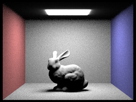
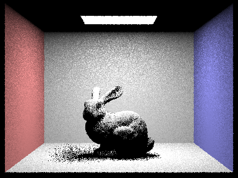
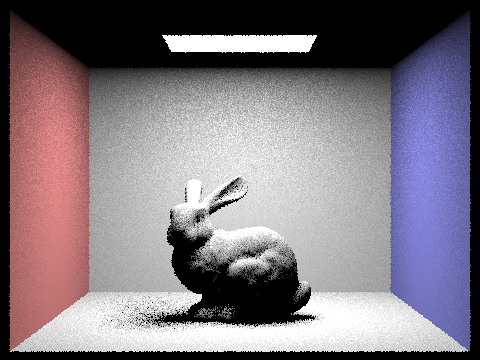
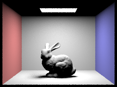
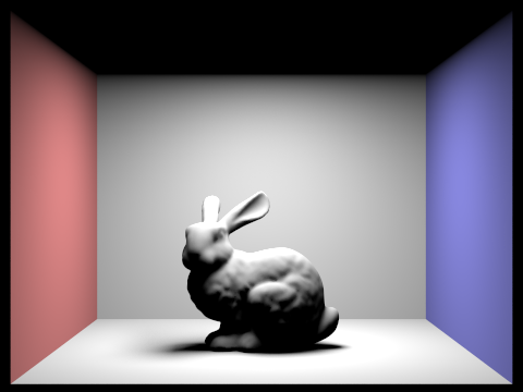
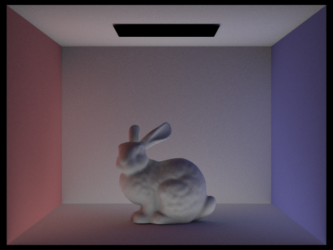
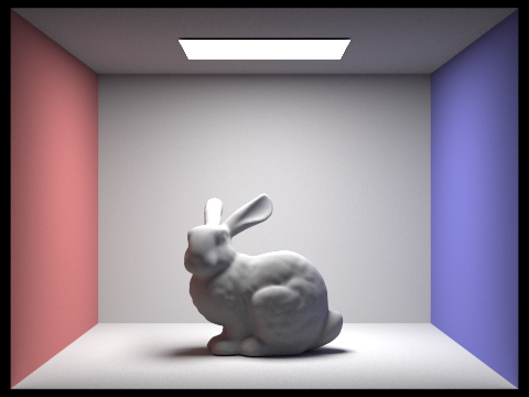
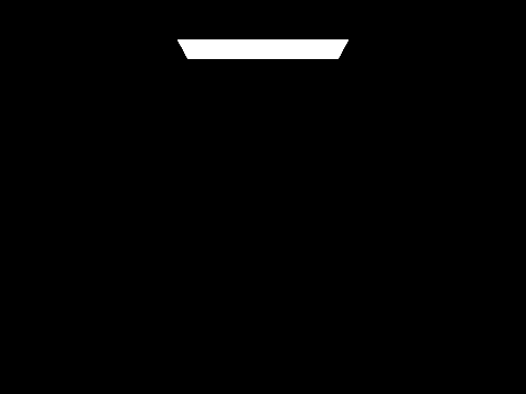
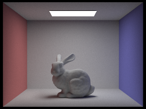
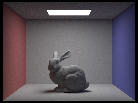
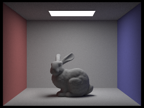
These images show the bunny.dae render using different amount of light rays with one sample using the direct lighting importance method. Focusing on the bunny's shadow, each iteration causes the shadow be to become less scattered.
In all the images that use uniform hemisphere sampling, there is a lot noise and disruptancies. This becomes more prevelant with scenes that have more complex lighting or highly directional light sources. In contrast, importance sampling focuses on sampling light sources based on their contribution to the scene. This results in images that have reduced noise and more accurate renderings with better convergence properties. An example of this is best shown with bunny.dae above where the background for the bunny on the left is very grainy and the light above seems to blur compared to bunny.dae on the right which has basically no noise and the subjects in the image are crisp.
Global illumination requires recursive calls on itself in order to account for the sum of indirect and direct lighting.
As direct lighting had been implemented in the previous part, we shall turn our attention to
indirect lighting. Below is a good visualizer for indirect lighting, where we continuously sample rays
from the first surface intersection to the second surface intersection in order to obtain how much radiance
the second surface is able to contribute to the first. In each recursive call, our new ray's origin is the previous
ray's surface intersection, and our new ray's direction is generated randomly from the sample_f function.
In order to find the amount of light shone upon a particular surface, we add the contribution of light from another surface's L_out scaled by the Monte-Carlo estimator
We pass in the maximum ray depth as an argument, and initialize the ray's depth to be the maximum ray depth. For each recursive call,
we define L_out to be the above, and include the next ray's L_out contribution and current ray's direct lighting contribution.
We decrease the ray depth by 1, and stop recursion once the ray depth becomes 1, or if there the next ray does not intersect
with a primitive. Other helper functions we used throughout
the implementation include sample_f - which samples using the input weight and returns the evaluation of the BSDF at the updated input.
|
|
|
|
|
|
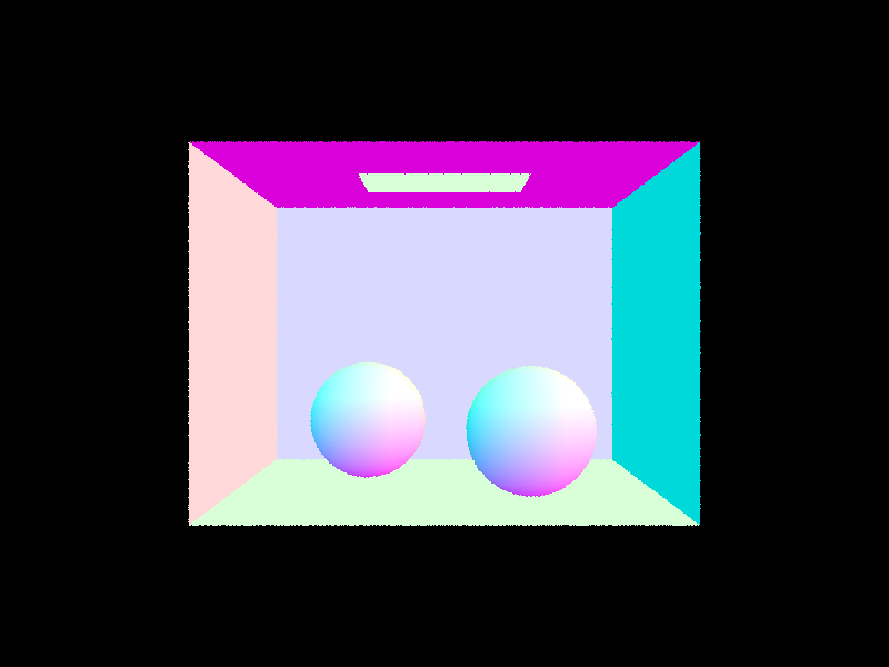
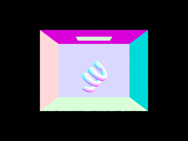
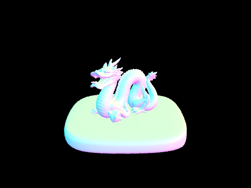
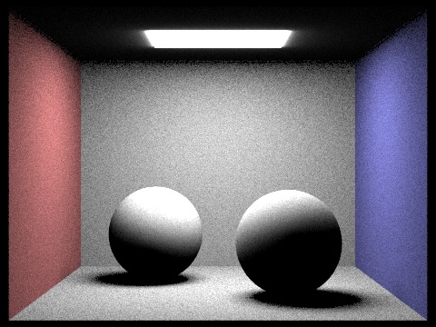
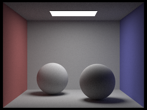
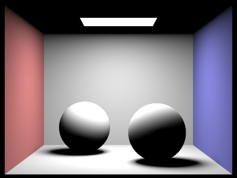
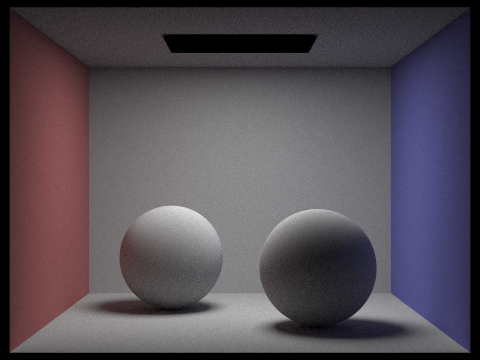
Comparison between indirect and direct illumination on the CBspheres_lambertian.dae file. To the left, we can see that for direct illumination, there is no bounce light from the primitives onto each other (the shadows appear black if it does not intersect with the light). In the right image, we can see the indirect reflection of light within the shadows of the spheres - the red wall bounces off red light and shines on the shadow of the left sphere, and the blue wall bounces off and shines on the shadow of the right sphere. This is rendered using a max ray depth of 4.
|
|
|
|
|
|
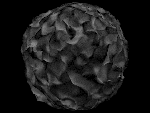
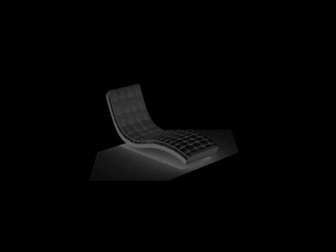
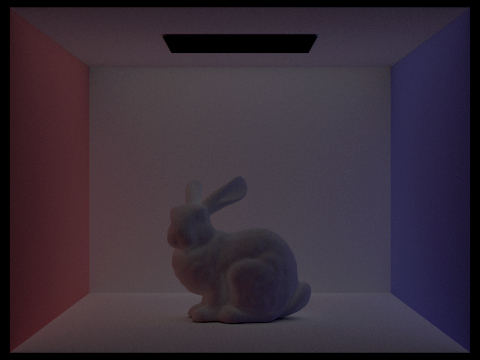
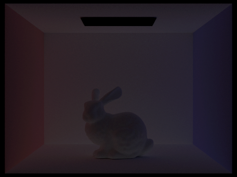
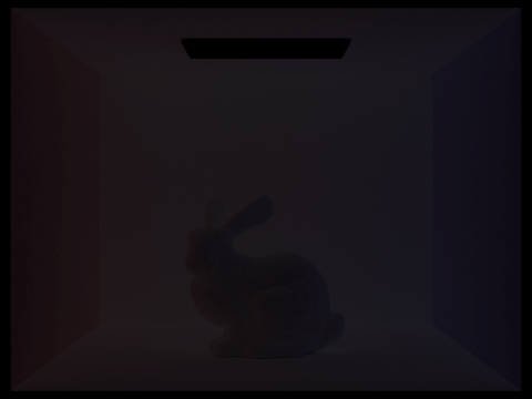
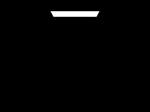
We also provided support for rendering only the mth bounce of light rather than the accumulation of all light from m recursive calls.
This can be toggled by setting the isAccumBounces parameter to false. Above are comparisons of each mth bounce of light.
Although this feature seems simple to implement, we spent a bit of time debugging. One issue was that the top of the spheres seemed to be
illuminated still. This was solved by immediately returning 0 light contribution when there was no intersection with another surface.
In the second and third bounce of light, we can note drastic changes in the exposure of the image. The render with a max_ray_depth of 2 appears brighter than that with a max_ray_depth of 3. However, the render with a max_ray_depth of 3 appears softer than 2. Using sampling from ray-tracing as opposed to rasterization leads to a more physically accurate result for the render, and can soften shadows naturally with a greater max_ray_depth, but rasterization can lead to quicker results, albeit not as accurate with the shape of the model and lights being taken into account.
|

|

|
|

|

|
We can see as we reach higher ray depths, there is less of a difference in the quality and appearance of the image.
|

|
|

|
|
|
The implementation of Global Illumination with Russian Roulette. We can choose to randomly terminate
the recursion for raytracing with a probability of ~0.35 for any given pixel, and also divide by this probability
in our Monte-Carlo estimator. This method prevents
bias in our estimator for global illumination. We used the built-in coin_flip(float probability)
function to determine whether we want to continue raytracing or not for a given pixel. With this, we are able to
render even an image with a max ray depth of 100 as quickly as an image with a max ray depth of 4 without Russian Roulette
in place.
|
|
|

|

|

|

|
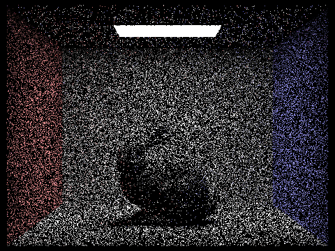
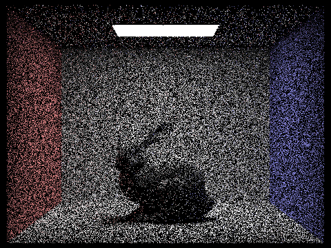
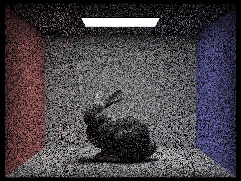
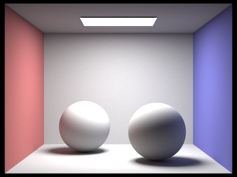
With 4 light rays and a max_ray_depth of 5, our output image appears less noisy when the sample size increases. This is because with an increase of samples, we can converge to a better predictor of the actual amount of light beign shone on a particular pixel.
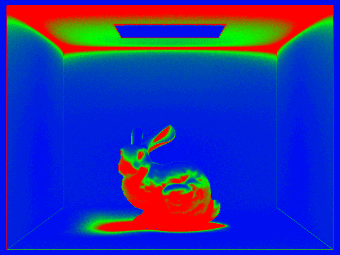
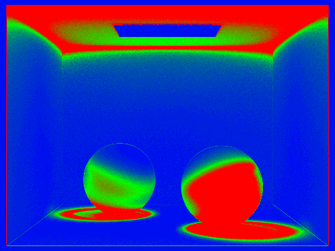
Our adaptive sampling method uses a confidence interval in order to terminate sampling for pixels that converge early when estimating their illuminance. The following formula for the confidence interval is given by \(I = 1.96 \cdot \frac{\sigma}{\sqrt{n}}\). Thus, as we collect more samples, our standard error decreases, and so does \(I\). We define our converging value to be \(I \leq \text{maxTolerance} \cdot \mu\). We will put the number of samples when a particular pixel converges in sample buffer.
Since we only need to keep information about the standard deviation, reoccuring number of samples, and the mean illuminance of the pixel, we keep these relevant values: \(\mu = \frac{s_1}{n} \) and \(\sigma = \frac{1}{n-1} (s_2 - \frac{s_1^2}{n}) \) where \( s_1 = \frac{1}{n} \sum_{k=1}^{n} x_k \) and \( s_2 = \frac{1}{n} \sum_{k=1}^{n} x_k^2 \). These values are then used to compute the standard error and mean of the pixel's illuminance. After defining these variables, the code is meant to shortcircuit once the \(I \leq \text{maxTolerance} \cdot \mu\) as we stop tracing more rays for the pixel after every 32 samples. The reason why we check for convergence every 32 samples is because it would be too costly to check every for every increase in 1 sample.
|

|
|
|
We both split up the work equally, but mostly Mahum started off writing the base code while Rebecca debugged. We both went to office hours and did equal parts of the writeup. Rebecca rendered all the images on her computer. Since both of us had a midterm the day before the project was due, we implemented part 1 and half of part 2 before the midterm, and did everything else after. Throughout this entire project, we learned a lot about raytracing techniques, how rays are transformed from various coordinate systems, and the fact that Mahum's computer is slow at rendering :( . While debugging, we often had to go back to previous commits, and learned how to create new branches in GitHub and merge them in the process.